Pump Curve Correction Calculator: Speed, Impeller, Density & Viscosity Adjustments
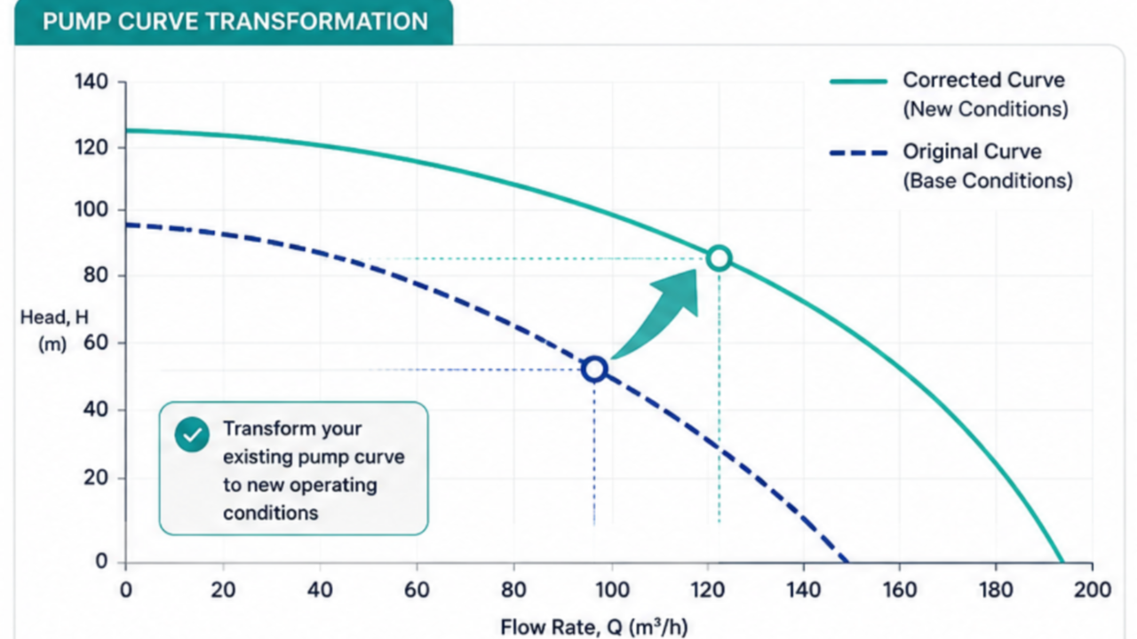
A centrifugal pump's published curve is measured on water at one speed and one impeller diameter. This tool re-draws that curve for a different speed or a trimmed impeller using the affinity laws, recomputes shaft power for the actual fluid density, and — when the fluid is more viscous than water — applies the ANSI/HI 9.6.7 viscosity correction. You choose which of those effects to apply; everything else is left untouched.
On this page
1 · The base curve 2 · Speed change 3 · Impeller diameter NPSHr 4 · Density & power 5 · Viscosity (HI 9.6.7) Worked example References
Enter the manufacturer pump curve as a set of flow–head points. Efficiency is optional: it is used only to compute shaft power and to locate the best efficiency point (BEP) for the viscosity method. If you only have a set of Q–H points, the affinity and density transformations still work — efficiency and power columns simply read as blank.
You then select what to transform: speed, impeller diameter, density, viscosity, or any combination. Only the inputs for the boxes you tick appear, so a job that is purely a density or viscosity question never asks for a speed or a diameter.
For a fixed impeller, changing rotational speed from N₁ to N₂ moves every point on the curve in fixed proportions: flow scales linearly with speed, head with the square, and power with the cube.[1]
Each entered point is scaled by these ratios to build the new curve. Speed predictions are accurate across a wide range, because the impeller geometry is unchanged.[2]
Trimming the impeller from D₁ to D₂ follows the same proportional pattern as speed, and the two effects multiply. When both change together the tool uses the combined ratio.[1]
H₂ / H₁ = [(N₂D₂) / (N₁D₁)]²
P₂ / P₁ = [(N₂D₂) / (N₁D₁)]³
If you enter NPSHr values with the curve, the tool scales them with the square of the speed ratio — the common approximation NPSHr₂ / NPSHr₁ ≈ (N₂ / N₁)².[10] This is the one transformation in the tool that should be trusted least.
A centrifugal pump develops head. Head expressed in metres of fluid is independent of density — a denser liquid does not change the Q–H curve. The efficiency curve is likewise unaffected by density; what density changes is the shaft power.[7] Selecting the density box recomputes power for the specified specific gravity while leaving head and efficiency untouched.
Under affinity scaling, corresponding points on the old and new curves share the same efficiency, so efficiency is carried across unchanged.[3] Shaft power at each point follows from the hydraulic power divided by efficiency.[4]
with Q in m³/h, H in m, g = 9.81 m/s², SG = ρ/1000 and η as a fraction. This is the standard hydraulic-power relation Pₕ = ρgQH divided by pump efficiency.[4]
More viscous fluids lower a pump's flow, head and efficiency relative to its water curve. The Hydraulic Institute method condenses the effect into a single dimensionless performance factor, parameter B, built from viscosity, BEP flow, BEP head and operating speed.[5][6] The tool evaluates B at the (already speed/diameter-scaled) BEP, so the correction is applied to the right operating point.
Evaluated in US units internally: ν in cSt, HBEP in feet per stage, QBEP in US gpm, N in rpm. A dynamic-viscosity input in cP is first converted with ν = μ / SG.[8]
Parameter B sets the flow factor Cₒ and the efficiency factor Cḱ. The head factor CḤ depends on where you are on the curve: it equals Cₒ at the BEP and moves toward 1 at lower flows and below Cₒ at higher flows. The closed-form equations are reproduced openly in the published literature.[5][8]
Cḱ = B(−0.0547 · B0.69)
CḤ = 1 − (1 − Cₒ) · (Q / QBEP)0.75
Each water point is mapped to its viscous equivalent: flow by Cₒ, head by CḤ at that flow, efficiency by Cḱ. Shaft power is then recomputed from the corrected flow, head and efficiency.
Take a water test curve with its BEP at 75 m³/h, 39 m, 72%. Slow the pump from 1750 to 1450 rpm and pump an oil of SG 0.90 at 200 cP. Two transformations apply in sequence: affinity scaling for speed, then the HI viscosity correction.
Speed ratio N₂/N₁ = 1450 / 1750 = 0.8286. At the BEP: flow 75 × 0.8286 = 62.1 m³/h; head 39 × 0.8286² = 26.8 m; efficiency unchanged at 72%.
Kinematic viscosity ν = 200 / 0.90 = 222 cSt. With the scaled BEP (62.1 m³/h, 26.8 m) at 1450 rpm, parameter B = 6.43, giving Cₒ = 0.919, CḤ = 0.919 at the BEP and Cḱ = 0.692.
| Quantity at BEP | Water, 1750 rpm | Scaled, 1450 rpm | + Viscous |
|---|---|---|---|
| Flow (m³/h) | 75.0 | 62.1 | 57.1 |
| Head (m) | 39.0 | 26.8 | 24.6 |
| Efficiency (%) | 72.0 | 72.0 | 49.9 |
| Shaft power (kW) | — | — | 6.91 |
| NPSHr (m) | 3.60 | 2.47 | 2.47 |
Shaft power is shown for the final viscous duty (SG 0.90): P = 0.90 × 9.81 × 57.1 × 24.6 / (3600 × 0.499) ≈ 6.91 kW. These figures match the live calculator's transformed-curve table exactly.
- Affinity Laws for Pumps — The Engineering ToolBox.
- Affinity Laws Made Simple — reliability limited to about a 10% impeller-diameter change because the casing/volute size is unchanged — Wilo Pump Basics; see also McNally Institute.
- Affinity Laws for Pumps — The Engineering ToolBox.
- Pump Power Calculator (hydraulic and shaft power) — The Engineering ToolBox.
- Effect of Viscosity on Pump Performance (parameter B method) — Campbell Tip of the Month.
- ANSI/HI 9.6.7 — Rotodynamic Pumps Guideline for Effects of Liquid Viscosity on Performance — Hydraulic Institute; plain-language summary at Pumps & Systems.
- Specific Gravity and Viscosity — specific gravity affects only the input power, not the head or efficiency curves — Pumps & Systems.
- Buratto et al., GPPS conference paper (prints the open-access HI parameter-B and CQ, CH, Cη equations) — Global Power & Propulsion Society (PDF).
- Lang, Satish & Berten, “Understanding Uncertainties in Viscous Performance Predictions for Centrifugal Pumps” (states the B < 40, 1–4000 cSt and radial-type validity limits) — Texas A&M Turbomachinery Laboratory (PDF).
- Elsey, “NPSHr Doesn’t Play by the Rules” (NPSHr scales roughly with speed squared but not cleanly; trim and speed both warrant supplier confirmation) — Pumps & Systems.
Estimates for preliminary engineering and screening. Confirm final selection with vendor data and a detailed analysis. Not a substitute for review by a qualified engineer.
Receive Free Discounts!
Join our mailing list to receive the latest engineering blogs, tools, resources and discounts on courses.
Don't worry, your information will not be shared.
Author